今日の高速デジタル環境では、データ転送速度はメガビット/秒、ギガビット/秒の単位で測定されます。8Kビデオのストリーミング、クラウドコンピューティング、メタバース、リアルタイム人工知能など、あらゆる分野で、ますます高速で信頼性の高い接続が求められています。
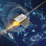
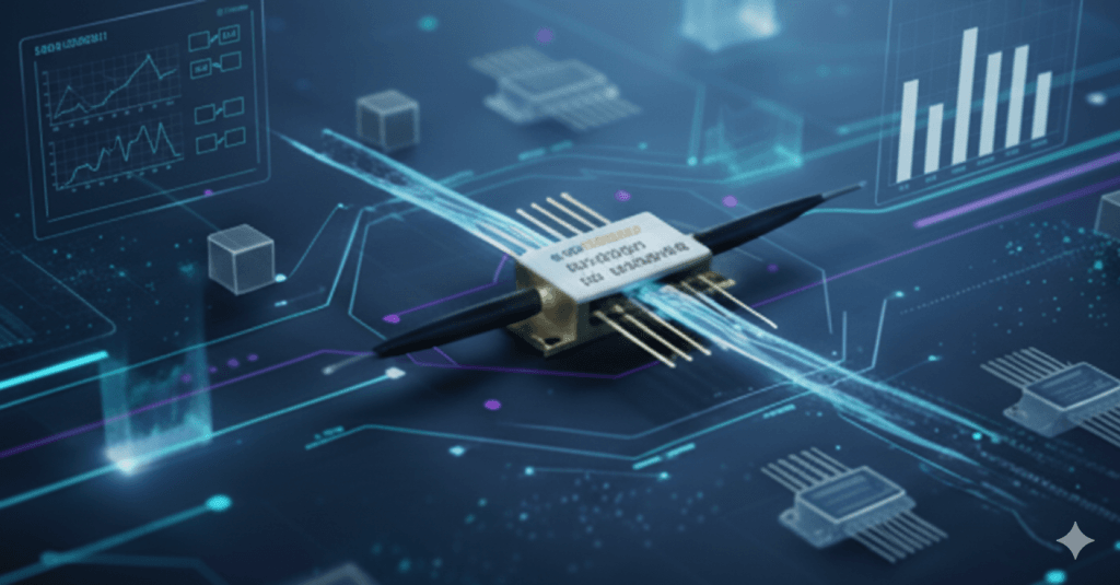
スーパールミネッセント・ダイオード(SLD)の一種である超広帯域SLEDなどの新デバイスは、ネットワーク機能の拡張に不可欠なツールとして台頭しています。INPHENIXのようなメーカーは最前線に立ち、120nmを超える帯域幅を備えた製品を提供することで、光通信の新たな性能基準を確立しています。
スピードへの飽くなき要求:帯域幅が重要な理由
高解像度メディア、仮想現実、拡張現実、没入型環境の出現によりデータのニーズが新たな高みに達するにつれ、ネットワーク使用量が増加しています。
クラウド コンピューティングと AI サービスには、超低遅延と高速データ交換が求められますが、数十億の IoT デバイス、RF テクノロジの統合、リモート ワークとリモート教育への移行により、この課題はさらに複雑になっています。
大規模シミュレーションやゲノム配列解析などの科学研究でも、膨大な量のデータが消費されます。
古い銅線システムと初期の光ファイバーシステムは現在、限界に直面しています。
光通信はこれらの課題を克服する必要があり、超広帯域 SLED は実行可能なソリューションを提供します。
超広帯域SLED:光通信の新たなパラダイム
スーパールミネッセント ダイオードは、増幅された自然放出光を利用して、コヒーレント レーザーと非コヒーレント LED 間のギャップを埋めます。
これらは、空間コヒーレンスが低く、パワーと明るさに優れた幅広い光スペクトルを生成します。
「超広帯域」というラベルが付いている場合、スペクトルは通常 50 nm ~ 100 nm の幅に拡張されますが、INPHENIX製品では 120 nm を超えることもあります。
広いスペクトルは、独立した各波長が独自のデータ ストリームを伝送できるように波長分割多重 (WDM)チャネルを増やすことで、より高いデータ容量をサポートします。
低コヒーレンスにより、レイリー後方散乱やクロストークなどの問題が軽減され、よりクリーンな長距離伝送が可能になります。
フラットで幅広いスペクトルは、ネットワーク設計者に次のようなメリットも提供します。
- チャネル割り当てとシステム再構成の柔軟性。
- システムの堅牢性が向上しました。
- 従来のレーザーに比べてモードノイズが最小限に抑えられます。
高速インターネットインフラにおける超広帯域SLEDの主な用途
大容量光ファイバー伝送システム
高密度波長分割多重(DWDM)は、現代のインターネットバックボーンの中核を成しています。超広帯域SLEDは、セグメント化したり、複数の安定したチャネルを生成したりできる広帯域シードを提供します。
これにより、単一のファイバーのデータ容量が増加し、テラビット/秒の速度がサポートされます。
120 nm を超える帯域幅を備えたINPHENIXの製品は、追加のファイバー インストールを必要とせずに、より多くのチャネルとデータ レートを実現します。
ネットワーク監視のための高度な光時間領域反射率測定法(OTDR)
OTDR システムは、ケーブル上の障害、減衰、破損箇所を特定することでファイバーの整合性を追跡します。
超広帯域SLEDの短いコヒーレンス長と広いスペクトルは、空間分解能とダイナミックレンジを向上させます。これにより、障害検出が迅速化され、ネットワークのダウンタイムが最小限に抑えられます。
継続的な高速インターネット アクセスを維持するためには、ネットワーク監視における正確な診断が不可欠です。
データセンターおよびネットワークノード内の光センシング
大規模なデータセンターでは、最適なパフォーマンスを維持するために正確な監視が必要です。
超広帯域 SLEDを使用した光センシングにより、複雑な環境内での温度、歪み、セキュリティをリアルタイムで監視できます。
これらのパフォーマンスにより、データセンターが効率的に運用され、コストのかかる障害を回避し、重要なインフラストラクチャのセキュリティと安定性が強化されます。
次世代パッシブ光ネットワーク(PON)
光ファイバー/構内展開におけるギガビットおよびテラビットの接続性の需要が高まるにつれ、現在の PON テクノロジには大幅なアップグレードが必要になります。
超広帯域 SLED は、より高密度の WDM-PON アーキテクチャをサポートしたり、高度なコヒーレント PON システムの広帯域ソースとして機能したりできます。
スペクトルの多様性により、将来的な容量増加やネットワークの複雑化に備えてラストマイル接続を準備できます。
重要インフラ監視用光ファイバージャイロスコープ(FOG)
FOG は主にナビゲーションに使用されますが、RF 技術を使用して、光ファイバー ケーブルをサポートする設備の微細な構造変化を監視したり、主要なデータ コンジット付近の地震活動を追跡したりすることもできます。
超広帯域 SLED は、このような高感度測定に必要な安定した低コヒーレンス光源を提供します。
INPHENIXのようなプロバイダーからの信頼性の高いパフォーマンスにより、微細な変更も確実に検出され、ネットワークの整合性の維持に役立ちます。
量子通信と未来の暗号
量子鍵配布やその他の量子光子アプリケーションの研究では、広く低コヒーレンススペクトルを持つ光源が役立ちます。
超広帯域 SLED は、近い将来、もつれ合った光子対を生成し、極めて安全なデータ伝送をサポートする実験で役割を果たす可能性があります。
この技術は、最終的には次世代の安全な通信ネットワークの基盤となる可能性があります。
INPHENIXが先導:超広帯域SLEDの限界を押し広げる
高品質な製造が、これらのアプリケーションの可能性を最大限に引き出す鍵となります。
INPHENIXは、120nmを超える帯域幅を持つ、高度な超広帯域SLED (超広帯域SLDとも呼ばれる)を製造しています。このスペクトル容量の増加により、既存の光ファイバーを介したWDMチャネル数の増加と、総データスループットの向上が可能になります。
製造プロセスでは次の点を重視しています。
- 安定性。
- 信頼性。
- 24時間のパフォーマンス。
波長、電力、パッケージをカスタマイズできるため、さまざまなシステム要件を満たすことができます。
半導体材料、フォトニック統合、RF、パッケージング技術の継続的な進歩により、パフォーマンスとコストの比率が継続的に向上し、重要なネットワーク アプリケーションでの展開が簡素化されます。
課題と今後の道筋
広く普及するには、いくつかの課題が残っています。
- メーカーは、高性能デバイスをコスト効率よくスケーラブルに生産する必要があります。
- 共通の標準を確立することで、さまざまなネットワーク間での相互運用性がサポートされます。
- これらの新しい光源を既存の広大なインターネット インフラストラクチャに統合するには、慎重なインターフェイスの設計と計画が必要です。
- ネットワークが拡大し、ますます広い地理的領域をカバーするようになるにつれて、電力の最適化は重要になります。
現在の研究は、超高速光ネットワークへのスムーズな移行を確実にするために、これらの側面を改善することに重点を置いています。
情報スーパーハイウェイを照らす
より高速なインターネットへの需要は、デジタル変革によって推進される永続的な変化です。
超ブロードバンド SLED は、データ容量の増加、ネットワークの整合性の確保、次世代の通信テクノロジーの実現に重要な役割を果たします。
マルチテラビット ネットワークとほぼゼロの遅延が一般的になるにつれ、高度なスーパールミネッセント ダイオードが、グローバルな接続性を維持するための中核となるでしょう。
INPHENIXのような業界リーダーが120 nm を超える帯域幅のデバイスを供給しているため、当社のネットワーク インフラストラクチャは将来のデータ負荷と進化するデジタル エクスペリエンスに適応する準備ができています。
これらの堅牢な光源は、拡張性の向上と柔軟な波長割り当てをサポートすると同時に、新たな課題と機会に向けてグローバル通信を準備します。