超辐射发光二极管(SLD)是边发射半导体光源。超辐射发光二极管(SLD)的独特特性是与输出激光二极管(LD)类似的高输出功率和低光束发散度,但具有更宽的光谱和低相干性,类似于发光二极管(LED)。超辐射发光二极管(SLD)在几何形状上与激光器类似,但是没有内置的LD反射机制用于受激发射以实现激光。与LD相比,超辐射发光二极管(SLD)操作的主要区别是:有源区内的增益更高,电流密度更高,光子的不均匀性和载流子密度分布更强。超辐射发光二极管(SLD)具有与LED相似的结构特征,通过降低刻面的反射率来抑制激光作用。超辐射发光二极管(SLD)本质上是高度优化的LED。虽然超发光二极管(SLD)像低电流水平的LED一样工作,但是它们的输出功率在高电流下也是超线性地增加。用于表征超辐射发光二极管(SLD)的六个关键参数:(1)输出功率;(2)光学增益; (3)ASE频谱带宽或3dB带宽; (4)频谱调制深度或纹波; (5)相干长度; 和(6)相干函数。
| 中心波长(nm) From: To: |
典型 3dB 带宽(nm) From: To: |
典型 输出 功率(mW) From: To: |
典型 波纹 (dB) | 典型 当前 From: To: |
封装类型 | 型号 |
|---|---|---|---|---|---|---|
| 中心波长(nm) | 典型 3dB 带宽(nm) | 典型 输出 功率(mW) | 典型 波纹(dB) | 典型 当前 | 封装类型 | 型号 |
| 750 | 10 | 3 | 0.1 | 120 | BUT或 DIL | |
| 750 | 14 | 10 | 0.1 | 120 | TO8、 9 或 56 前窗口 | |
| 770 | 13 | 8 | 0.1 | 180 | BUT或 DIL | |
| 770 | 20 | 5 | 0.1 | 140 | BUT或 DIL | |
| 780 | 12 | 3 | 0.1 | 150 | BUT或 DIL | |
| 780 | 12 | 10 | 0.1 | 180 | BUT或 DIL | |
| 780 | 40 | 5 | 0.1 | 200 | BUT或 DIL | |
| 800 | 10 | 15 | 0.1 | 200 | BUT或 DIL | |
| 800 | 40 | 5 | 0.1 | 200 | BUT或 DIL | |
| 820 | 15 | 0.3 | 0.1 | 120 | BUT或 DIL | |
| 820 | 15 | 5 | 0.1 | 120 | TO8、 9 或 56 前窗口 | |
| 820 | 15 | 8 | 0.1 | 140 | TO8、 9 或 56 前窗口 | |
| 820 | 25 | 2.5 | 0.1 | 140 | 但或 DIL | |
| 820 | 25 | 8 | 0.1 | 140 | 到 8、 9 或 56 前窗口 | |
| 820 | 40 | 5 | 0.1 | 180 | BUT或 DIL | |
| 830 | 30 | 15 | 0.2 | 200 | BUT或 DIL | |
| 830 | 32 | 45 | 0.1 | 250 | 到 8、 9 或 56 前窗口 | |
| 830 | 40 | 7 | 0.1 | 200 | BUT或 DIL | |
| 830 | 40 | 10 | 0.1 | 150 | 到 8、 9 或 56 前窗口 | |
| 830 | 50 | 5 | 0.1 | 150 | BUT或 DIL | |
| 840 | 35 | 5 | 0.1 | 160 | BUT或 DIL | |
| 840 | 45 | 8 | 0.1 | 200 | BUT或 DIL | |
| 840 | 45 | 11 | 0.1 | 250 | BUT或 DIL | |
| 840 | 50 | 8 | 0.1 | 200 | BUT或 DIL | |
| 850 | 50 | 8 | 0.1 | 200 | BUT或 DIL | |
| 870 | 50 | 6 | 0.1 | 180 | BUT或 DIL | |
| 880 | 45 | 6 | 0.1 | 200 | BUT或 DIL | |
| 880 | 40 | 2 | 0.1 | 180 | BUT或 DIL | |
| 880 | 45 | 8 | 0.1 | 180 | BUT或 DIL | |
| 880 | 55 | 5 | 0.1 | 180 | BUT或 DIL | |
| 900 | 15 | 20 | 0.2 | 200 | BUT或 DIL | |
| 900 | 15 | 35 | 0.2 | 200 | 到 8 或 9 前窗口 | |
| 900 | 30 | 10 | 0.1 | 200 | 到 8 或 9 前窗口 | |
| 900 | 45 | 7 | 0.1 | 200 | BUT或 DIL | |
| 920 | 30 | 3 | 0.1 | 150 | BUT或 DIL | |
| 920 | 55 | 8 | 0.1 | 200 | BUT或 DIL | |
| 920 | 90 | 5 | 0.1 | 200 | BUT或 DIL | |
| 980 | 25 | 5 | 0.1 | 250 | BUT或 DIL | |
| 1020 | 100 | 10 | 0.15 | 250 | BUT或 DIL | |
| 1020 | 60 | 7 | 0.1 | 150 | BUT或 DIL | |
| 1020 | 110 | 8 | 0.1 | 300 | BUT或 DIL | |
| 1040 | 55 | 30 | 0.2 | 400 | BUT或 DIL | |
| 1040 | 70 | 10 | 0.1 | 250 | BUT或 DIL | |
| 1050 | 45 | 35 | 0.2 | 400 | BUT或 DIL | |
| 1050 | 55 | 15 | 0.1 | 300 | BUT或 DIL | |
| 1050 | 55 | 30 | 0.1 | 400 | BUT或 DIL | |
| 1070 | 60 | 5 | 0.1 | 500 | BUT或 DIL | |
| 1070 | 60 | 10 | 0.15 | 400 | BUT或 DIL | |
| 1280 | 55 | 10 | 0.5 | 350 | BUT或 DIL | |
| 1280 | 70 | 5 | 0.15 | 300 | BUT或 DIL | |
| 1280 | 95 | 10 | 0.5 | 500 | BUT或 DIL | |
| 1310 | 40 | 1.5 | 0.1 | 120 | 到 8、 9 或 56 前窗口 | |
| 1310 | 40 | 0.5 | 0.1 | 120 | 到 56 尾纤前纤维 | |
| 1310 | 40 | 5 | 0.1 | 150 | 到 8、 9 或 56 前窗口 | |
| 1310 | 40 | 35 | 1 | 400 | BUT或 DIL | |
| 1310 | 45 | 1 | 0.1 | 120 | BUT或 DIL | |
| 1310 | 45 | 20 | 1 | 350 | BUT或 DIL | |
| 1310 | 45 | 25 | 1 | 350 | BUT或 DIL | |
| 1310 | 50 | 15 | 0.2 | 150 | 到 8、 9 或 56 前窗口 | |
| 1310 | 55 | 7 | 0.5 | 300 | 但或 DIL | |
| 1310 | 55 | 20 | 1 | 450 | BUT或 DIL | |
| 1310 | 55 | 25 | 1 | 350 | BUT或 DIL | |
| 1310 | 70 | 18 | 1 | 500 | BUT或 DIL | |
| 1310 | 65 | 15 | 1 | 250 | BUT或 DIL | |
| 1310 | 80 | 15 | 1 | 450 | BUT或 DIL | |
| 1310 | 90 | 10 | 1 | 350 | BUT或 DIL | |
| 1310 | 100 | 3 | 0.1 | 180 | BUT或 DIL | |
| 1410 | 50 | 10 | 1 | 300 | BUT或 DIL | |
| 1410 | 60 | 15 | 1 | 450 | BUT或 DIL | |
| 1410 | 70 | 10 | 1 | 550 | BUT或 DIL | |
| 1490 | 50 | 5 | 0.5 | 200 | BUT或 DIL | |
| 1490 | 65 | 18 | 1 | 500 | BUT或 DIL | |
| 1520 | 50 | 15 | 0.15 | 400 | BUT或 DIL | |
| 1520 | 75 | 10 | 1 | 350 | BUT或 DIL | |
| 1550 | 40 | 0.2 | 0.15 | 120 | 到 56 尾纤前纤维 | |
| 1550 | 55 | 0.5 | 0.1 | 120 | BUT或 DIL | |
| 1550 | 55 | 5 | 0.2 | 200 | BUT或 DIL | |
| 1550 | 60 | 3 | 0.2 | 300 | BUT或 DIL | |
| 1550 | 50 | 3 | 0.2 | 150 | 到 8、 9 或 56 前窗口 | |
| 1550 | 60 | 10 | 1 | 300 | BUT或 DIL | |
| 1550 | 65 | 12 | 0.15 | 300 | BUT或 DIL | |
| 1550 | 65 | 20 | 0.4 | 450 | BUT或 DIL | |
| 1550 | 90 | 8 | 1 | 300 | BUT或 DIL | |
| 1580 | 60 | 5 | 0.2 | 300 | BUT或 DIL | |
| 1580 | 75 | 5 | 0.4 | 300 | BUT或 DIL | |
| 1610 | 55 | 2 | 0.1 | 250 | BUT或 DIL | |
| 1610 | 55 | 5 | 0.5 | 250 | BUT或 DIL | |
| 1640 | 40 | 5 | 0.5 | 400 | BUT或 DIL | |
| 1640 | 50 | 3 | 0.5 | 200 | BUT或 DIL |
SLDs have been used for many different applications. The major application fields are
(1) Optical Coherence Tomography
(2) White light interferometry
(3) Fiber-optic link testing
(4) WDM PON systems
(5) Fiber-optic sensors
(6) Fiber-optic gyroscopes
The actual applications in each field are summarized in Table 1. More details are described in the following sections.
| Optical Coherence Tomography (OCT) |
|
800 nm band
1050 nm band 1310 nm band
|
| White light interferometry |
|
800 nm band
1310 nm band 1550 nm band |
| Fiber-optic link testing |
|
1310 nm band
1550 nm band |
| WDM PON systems |
|
1550 nm band |
| Fiber-optic sensors |
|
1550 nm band |
| Fiber-optic gyroscopes |
|
800 nm band
1550 nm band |
Optical coherence tomography (OCT) is an optical signal acquisition and processing method using an interferometric technique to capture micrometer-resolution, three-dimensional images from within optical scattering media such as biological tissue. SLDs have been used as a broad-band spectrum light source. Very wide-spectrum emitting over a ~100nm wavelength range have achieved sub-micrometer resolution. Optical coherence tomography typically employs near infrared light. The use of relatively long wavelength light allows it to penetrate into the scattering medium.
Commercially available optical coherence tomography systems are employed in diverse applications, including art conservation and diagnostic medicine, notably in ophthalmology where it can be used to obtain detailed images from within the retina. Recently it has also begun to be used in interventional cardiology to help diagnose coronary artery disease.
There are two types of OCT: (1) Time-domain OCT, and (2) Frequency-domain OCT.
(a) Time-domain OCT :
Basic configuration of time–domain OCT system is shown in Fig. 1 [1]. Light in an OCT system is broken into two arms—a sample arm (containing the item of interest) and a reference arm (usually a mirror). The combination of reflected light from the sample arm and reference light from the reference arm gives rise to an interference pattern, but only if light from both arms have travelled the “same” optical distance (“same” meaning a difference of less than a coherence length). By scanning the mirror in the reference arm, a reflectivity profile of the sample can be obtained.
The axial and lateral resolutions of OCT are decoupled from one another; the former being an equivalent to the coherence length of the light source and the latter being a function of the optics. The coherence length of a source and hence the axial resolution of OCT is defined as,
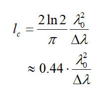
where Δλ is the 3dB bandwidth of the SLD spectrum, and λ0 is the central wavelength.
(b) Frequency-domain OCT :
In frequency domain OCT, the broadband interference is acquired with spectrally separated detectors, either by encoding the optical frequency in time with a spectrally scanning source or with a dispersive detector, like a grating and a linear detector array. One example of the frequency-domain OCT configuration with using a spectrally scanning source, is shown in Fig. 2 [2]. Due to the Fourier relation (Wiener-Khintchine theorem between the auto correlation and the spectral power density), the depth scan can be immediately calculated by a Fourier-transform from the acquired spectra, without movement of the reference arm. This feature improves imaging speed dramatically, while the reduced losses during a single scan improve the signal to noise proportional to the number of detection elements. The parallel detection at multiple wavelength ranges limits the scanning range, while the full spectral bandwidth sets the axial resolution.


White light interferometry is to capture intensity data at a series of positions along the vertical axis where the surface is located by using the shape of the white-light interferogram, the localized phase of the interferogram, or a combination of both shape and phase.
An example of the operation principle is illustrated in Fig. 3. The light of a broadband light source (SLD) with short coherence length is split into two beams: an object beam and a reference beam. The object beam reflects from the object (sample), and the reference beam reflects off of a reference mirror. The two reflected beams are captured and recombined at the beam splitter. The superimposed beams are imaged by a CCD camera for processing. If the optical path for an object point in the measurement arm is the same as the optical path in the refrence arm, there is constructive interference, which results in a high intensity in the camera pixel of the respective object point, for all wavelengths in the spectrum of the SLD. For object points having a different optical path, the interference is destructive, which results in a much lower intensity. In this way, the topolographical structure of the sample is converted to light intensity difference, and, therefore, to the CCD output signals, which are compiled and analyzed.
One example of white light interferometry application is to measure the surface roughness on semiconductor wafers [3].

SLDs are used in the diagnostics of optical fiber communication networks in the 1310nm and 1550nm bands. The chromatic dispersion of an optical medium is the phenomenon that the phase velocity and group velocity of light propagating in a transparent medium depend on the optical frequency. Dispersion has an important impact on the propagation of optical pulses, because a pulse always has a finite spectral width (bandwidth), so that dispersion can cause its frequency components to propagate with different velocities. Normal dispersion, for example, leads to a lower group velocity of higher-frequency components, and thus to a positive chirp, whereas anomalous dispersion creates negative chirps. The frequency dependence of the group velocity also has an effect on the pulse duration. If the pulse is initially unchirped, dispersion in a medium will always increase its duration (dispersive pulse broadening).
In optical fibers, there is usually some slight difference in the propagation characteristics of light waves with different polarization states. This is called polarization mode dispersion (PMD) [3]. A differential group delay can occur even for fibers that according to the design should have a rotational symmetry and thus exhibit no birefringence. This effect can result from random imperfections or bending of the fibers, or from other kinds of mechanical stress, and is also affected by temperature changes. Mainly due to the influence of bending, the PMD of a cabled fiber can be completely different from that of the same fiber on a spool. Modern fiber cables as used in fiber-optic links have been optimized for low PMD, but the handling of such cables can still have some influence. PMD can have adverse effects on optical data transmission in fiber-optic links over long distances at very high data rates, because portions of the transmitted signals in different polarization modes will arrive at slightly different times. Effectively, this can cause some level of pulse broadening, leading to inter-symbol interference, and thus a degradation of the received signal, leading to an increased bit error rate.
The chromatic dispersion and polarization mode dispersion (PMD) can be measured by using the large bandwidth, high power spectral density, and low ripple characteristics of SLDs.
The Wavelength Division Multiplexing (WDM) Passive Optical Networks (PON) has been used and developed as one of the approaches for Fiber To The Home (FTTH) network systems [5][6]. As a low-cost laser source at the Optical Network Unit (ONU) in such WDM PON systems, the Fabry Perot (FP) laser diode (LD) wavelength is locked to a selected wavelength channel of the broad-band Amplified Spontaneous Emission (ASE) source.[6]. Fig. 4 shows an architecture for upstream transmission employing wavelength-locked FP LDs [6]. A broad-band ASE source (such as SLD) with an optical circulator is located at the central office. The broad-band ASE is transmitted to the remote node where an Arrayed Waveguide Grating (AWG) slices the ASE spectrally. The spectrally sliced ASE is injected into the FP LD located at the ONU.

(a) Advantages of FOS
(b) Types of FOS
There are two types of fiber optic sensors:
(c) Intrinsic Sensors
The optical characteristics of an optical fiber is sensitive to the strain, temperature, and pressure, which modulates the intensity, phase, polarization, wavelength, or transit time of light in the fiber. A particularly useful feature of intrinsic fiber optic sensors is that they can, if required, provide distributed sensing over very large distances.
Optical fiber sensors for temperature and pressure have been developed for downhole measurement in oil wells. The fiber optic sensor is best suited for this environment as it functions at temperatures too high for semiconductor sensors (distributed temperature sensing).
Fiber-optic sensors have been developed to measure co-located temperature and strain simultaneously with very high accuracy using fiber Bragg gratings. This is particularly useful when acquiring information from small complex structures. Brillouin scattering effects can be used to detect strain and temperature over larger distances (20–30 kilometers). The fiber sensor is especially useful for harsh environments.
Example: Bragg grating sensors for strain and temperature
A schematic diagram of the fiber Bragg grating sensor is shown in Fig. 5.
The Bragg wavelength can be expressed as,
![]()
where n is the mode index of the fiber, and Λ is the grating period. Equation (1) gives,
![]()
where ΔλB, Δn and ΔΛ express a small change of λB, n, and Λ, respectively.

A fiber-optic AC/DC voltage sensor in the middle and high voltage range (100–2000V) can be created by inducing measurable amounts of Kerr nonlinearity in single mode optical fiber by exposing a calculated length of fiber to the external electric field. The measurement technique is based on polarimetric detection and high accuracy is achieved in a hostile industrial environment.
High frequency (5MHz–1GHz) electromagnetic fields can be detected by induced nonlinear effects in fiber with a suitable structure. The fiber used is designed such that the Faraday and Kerr effects cause considerable phase change in the presence of the external field. With appropriate sensor design, this type of fiber can be used to measure different electrical and magnetic quantities and different internal parameters of fiber material.
Electrical power can be measured in a fiber by using a structured bulk fiber ampere sensor coupled with proper signal processing in a polarimetric detection scheme. Experiments have been carried out in support of the technique.
Hydrophone systems with more than one hundred sensors per fiber cable have been developed. Hydrophone sensor systems are used by the oil industry as well as a few countries’ navies. Both bottom-mounted hydrophone arrays and towed streamer systems are in use.
Fiber optic microphone and fiber-optic based headphone find application in areas with strong electrical or magnetic fields, such as communication amongst the team of people working on a patient inside a magnetic resonance imaging (MRI) machine during MRI-guided surgery.
(d) Extrinsic Sensors
Extrinsic fiber optic sensors use an optical fiber cable, normally a multimode one, to transmit modulated light from either a non-fiber optical sensor, or an electronic sensor connected to an optical transmitter. A major benefit of extrinsic sensors is their ability to reach places which are otherwise inaccessible. Extrinsic fiber optic sensors provide excellent protection of measurement signals against noise corruption:
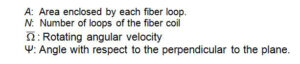
The interferometric fiber optic gyroscope (IFOG) uses an optical interferometer for the very high-resolution readout of the Sagnac phase shift induced between two counter-propagating waves in an optical closed path when the plane of propagation undergoes angular rotation. The basic scheme is illustrated in Fig. 6. It is a passive interferometer where the fiber optic coupler is employed to split the radiation from the light source into two counter-propagating waves, clockwise (CW) and counterclockwise (CCW), in the fiber coil and to recombine the waves, after propagation, on a photodetector PD. The phase difference is thus cumulated over a long fiber coil for obtaining high responsivity with a compact device. For ideal fibers and components, the output photo-generated current I has the following expression:
![]()
where φS is the so-called Sagnac phase shift, and

where σ is the photodetector responsivity and P is the power coupled into the input fiber.
The Sagnac phase shift φS is given by (see Fig.7),

![]()
where